Exercises
General
P.1
Given the following list:
l = ['a', 2, 7, 3.0, 4.5]
Using the print()-statement på print out the last item in the list without directly giving the last index in the list.
P.2
Given the following list:
l = [1, 2, 3, 4, 5, 6, 7]
Assign a new list l2 that contains all values except the first value in the list. The answer should be able to be applied to arbitrary lists. Print the response using print().
P.3
Given the list:
l = [67, 87, 34, 67, 99]
Assign a new list l2 that contains all items except the last and first values from L. Print the list with the print()-statement.
P.4
Given the list:
l = [67, 87, 34, 67, 99]
Add the value 100 to the last in the list.
P.5
Given the list:
l = [67, 87, 34, 67, 99]
Insert the value 52 first in the list.
P.6
Given the list:
l = [67, 87, 34, 67, 99]
Insert the value -27 between 87 and 34.
P.7
Given the list:
l = ["Arne", "Per", "Sven", "Nils", "Bill", "Per"]
Remove first occurrence of “Per”.
P.8
Given the list:
l = ["Arne", "Per", "Sven", "Nils", "Bill", "Per"]
Use the del function to remove “Sven”.
P.9
Given the following list:
l = ["Arne", "Per", "Sven", "Nils", "Bill", "Per"]
Delete the first two names in the list.
P.10
Create a nested list of five rows and six columns where all items have a value of 42. Use print() to print the value of the position (2,2).
P.11
Create a dictionary, phone_book, with the following keys and values:
Arne, 47329823
Bengt, 91238129
Stina, 1928319
Lena, 98129312
P.12
Enter the range() statement for the sequence 2, 5, 8
P.13
Type a for statement that iterates over the l:
l = [45, 78, 90, 34, 23]
Without using a range()-statement. Print each value in the list.
P.14
Create a for statement to iterate over the list in 13, but use a for loop with a range() function.
P.15
Write a for-statement that iterates over every other value in the list in task 13.
P.16
Write a program that summarizes values from the lists, a, and b. The sum from the lists shall be assigned to list c, which shall be the same length as a and b at the end of the programme. Print the list c.
a = [3, 6, 8, 10, 34, 32]
b = [76, 45, 10, 6, 89, 11]
Tip: Use the zip()-function.
P.17
Write a program that iterates and prints all the elements in the following nested list: nested_list = [[1, 2, 3], [4, 5, 6, 7, 8, 9], [10, 11]]
P.18
Write a program that iterates from 2 to 100 and for each number in the series and prints if it is a prime number or not.
If a number n is a prime number, it can be determined by dividing this by all numbers from 2 to sqrt (n). If any remnant of the division becomes 0, n is not a prime number. The remainder of a division can be determined using the modulo operator, %, in Python. Use break to cancel a loop when the rest becomes 0.
P.19
Convert the program in P. 18 to use a function that returns True if n is a prime number; otherwise False. Also, write code to calculate the prime numbers between 2 to 100 by iterating and calling the function.
P.20
Write a function that assigns all values in a list 0 if these are less than 0. To test the function, the following code can create a list of random numbers:
from random import randint
l = [randint(-100,101) for i in range(100)]
The randint(a, b)-function returns a random number k between a < = k < b. The list provided as an argument should be modified in place. The function should not return a new list.
P.21*
Functions can be given as an argument just like any other datatype in Python. Implement a function to differentiate numerically according to the formula:
The function should take a function as input and the parameters x and h. Write a main application that calls the function with f(x)=sin(x) and calculates f’(x) when x=2.0.
P.22*
Implement a function to create function tables of a particular function. The function shall, as input parameters, take the starting and ending values, stride length and the function to be plotted. An example of printing is shown below for the function f(x) = sin(x):
x f(x)
-6.2832 0.0000
-6.1832 0.0998
-6.0832 0.1987
-5.9832 0.2955
Use the .format()-function to print the formatting.
P.23*
Write the following list to file:
l = [
    [45, 78, 56, 34],
    [9, 23, 23],
    [34, 87],
    [12, 19, 78, 56, 45]
]
Each nested list should be written to a separate line, i.e. The final file must contain:
45 78 56 34
9 23 23
34 87
12 19 78 56 45
Use the with statement to ensure that .close() is called. Be aware that values must be converted to strings before they are written to the file. This can be done using the str()-function. A new line is obtained by using the. Write (“n”) method on the Object object.
P.24*
Write a program that loads the file from P.23 and stores the values in a list with the same structure. Text strings can be split with respect to spaces by using the method .split() method. Values stored in strings can be converted to values by using the int()-function.
P.25
In this example, we will open and read a CSV file with the outbreak data from a geyser. The file can be downloaded from:
https://github.com/jonaslindemann/guide_to_python/blob/master/exercises/faithful.csv.
The file begins with a “header” line and is followed by the data separated by commas into three columns according to:
"Index", "Eruption length (mins)","Eruption wait (mins)"
1, 3.600, 79
2, 1.800, 54
3, 3.333, 74
...
Type a function read_data(filename) that loads the CSV file and converts it into a nested list, where each row consists of a list of three values corresponding to the columns contained in the file. The function should return the header line and a list of the loaded data.
Type a function query_data(table, t), which extracts all rows in the table list that exceed T minutes in the outbreak time. The function returns a new list with the rows that exceed t; otherwise, the format is the same as the loaded list.
Type a function write_data(header, table, filename) that writes a new CSV file with the same structure as the loaded file.
Type a main program that loads faithful.csv, extracts outbreaks above 4.5 degrees, and writes the results to the faithful_max_4_5.csv file.
P.26
Add error handling routines to task P.24 and P.25.
NumPy
P.27
Create the following one-dimensional arrays in NumPy:
Integer array with the following content:
[1 2 3]
Floating-point array with the following appearance:
[1.0 2.0 3.0 4.0 5.0 6.0 7.0]
P.28
Create the following two-dimensional arrays in NumPy:
Integer array with the following appearance:
floating point arry with the following appearance:
P.29
Write code to print all information about the following array:
b = np.array([[1, 2, 3], [4, 5, 6]], float)
P.30
Change the shape of the following array to a one-dimensional array:
a = np.array([[1, 2, 3, 4, 5, 6], [7, 8, 9, 10, 11, 12]])
P.31
Create a new array b based on a with the 12 x 12 dimension.
a = np.array([[1, 2, 3, 4, 5, 6], [7, 8, 9, 10, 11, 12]])
P.32
Create a 5 x 5 floating-point array filled with zeros.
P.33
Create a 10 x 10 integer array filled with ones.
P.34
Create a 10 x 5 integer array in which all elements have a value of 27.
P.35
Create the following array by using the np.arange() function:
[[ 10 11 12 13 14]
 [ 15 16 17 18 19]
 [ 20 21 22 23 24]
 [ 25 26 27 28 29]
 [ 30 31 32 33 34]
 [ 35 36 37 38 39]
 [ 40 41 42 43 44]
 [ 45 46 47 48 49]
 [ 50 51 52 53 54]
 [ 55 56 57 58 59]
 [ 60 61 62 63 64]
 [ 65 66 67 68 69]
 [ 70 71 72 73 74]
 [ 75 76 77 78 79]
 [ 80 81 82 83 84]
 [ 85 86 87 88 89]
 [ 90 91 92 93 94]
 [ 95 96 97 98 99]
 [100 101 102 103 104]
 [105 106 107 108 109]]
The array can be created with a single statement in NumPy.
P.36
Create the following array with a single statement in NumPy.
[[1. 0. 0. 0. 0. 0.]
 [0. 1. 0. 0. 0. 0.]
 [0. 0. 1. 0. 0. 0.]
 [0. 0. 0. 1. 0. 0.]
 [0. 0. 0. 0. 1. 0.]
 [0. 0. 0. 0. 0. 1.]]
P.37*
Create an array of 100 values ranging from –π to π. Start and end values must be included in the array. The value of π can be obtained in NumPy with np.pi. (np is NumPy-import-prefix.)
P.38*
Given the following matrices:
A = np.random.randint(0, 100, [5, 5])
B = np.random.randint(0, 100, [5, 5])
Create a new array, C, which is the matrix multiplication of AB.
P.39*
Given the following array:
[[ 0 1 2 3 4 5]
 [ 6 7 8 9 10 11]
 [12 13 14 15 16 17]
 [18 19 20 21 22 23]
 [24 25 26 27 28 29]
 [30 31 32 33 34 35]]

# a = np.arange(36).reshape(6,6)
Write expression that returns:
the value of row 2, column 2
row 3
column 4
the last row
the last column
Matplotlib exercises
P.40
Plot np.sin(x), np.cos(x), np.tan(x) and np.arctan(x) in a single figure using the plt.subplot() command. Set suitable y-limits for the different plots and give each plot its own title.
P.41
Square waves can be formed by summing sine waves of odd harmonics. For example:
t = np.linspace(-2*np.pi, 2*np.pi)
y = np.sin(t) + np.sin(3*t)/3 + np.sin(5*t)/5 + np.sin(7*t)/7
Or as a sum of
np.sin(k*t)/k, where k = 1, 3, 5, 7, …
Plot all sums from k = 1 to k = 19 in a single plot Add labels and titles to the diagram.
P.42
Plot the function f(x,y) = sin(x*y/4.0) as a contour plot (plt.contour()) and a filled contour (plt.contourf()) plot in separate figures. Plot range should be from -2*pi to 2*pi in both x and y directions. Each plot should have 10 contour levels. Add labels and titles to the diagram.
P.43
Plot the function f(x,y) = sin(x*y/4.0) as a 3D surface. Plot range should be from -2*pi to 2*pi in both x and y directions. 3D surface plots can be created by adding the following imports:
from mpl_toolkits.mplot3d import axes3d
import matplotlib.pyplot as plt
from matplotlib import cm
An axes object has to be created to activate 3d-plotting in the current figure.
fig = plt.figure()
ax = plt.axes(projection='3d')
The ax.plot_surface() method can the be used to plot the surface. See also lecture slides and the documentation for plot_surface() in the matplotlib documentation.
Object-oriented Programming
P.45
Use the base classes from the lecture and implement a Rectangle class with the additional attributes width and height.
Implement a Polyline class that can handle a set of Point derived objects. The class should have methods for adding, removing and clearing the points. It should also have a methods or properties for accessing the Point-objects in the class.
All classes should implement the __str__() method for printing a description of the object. Write an example tha illustrates the use of your new classes.
Use the code from the lecture as a base for the assignment.
P.46
Implement a class, Geyser, which implements the functionality of assignment P.25. The class constructor should have an argument, filename, which is stored as a member variable self.filename. The constructor should also call the read_data() method to read data. read_data() function is implemented as a member function, reading the data and storing the read table as a member variable. The query_data() method takes single argument t (time of eruption) and returns a nested list of the eruptions longer than t.
The class should be able to be used like in the code below:
geyser = Geyser("faithful.csv")
print(geyser.data_table)
result_table = geyser.query_data(4.5)
print(result_table)
ParaView
Datafiles and additional python modules can be found here:
https://github.com/jonaslindemann/compute-course-public/tree/master/dataviz
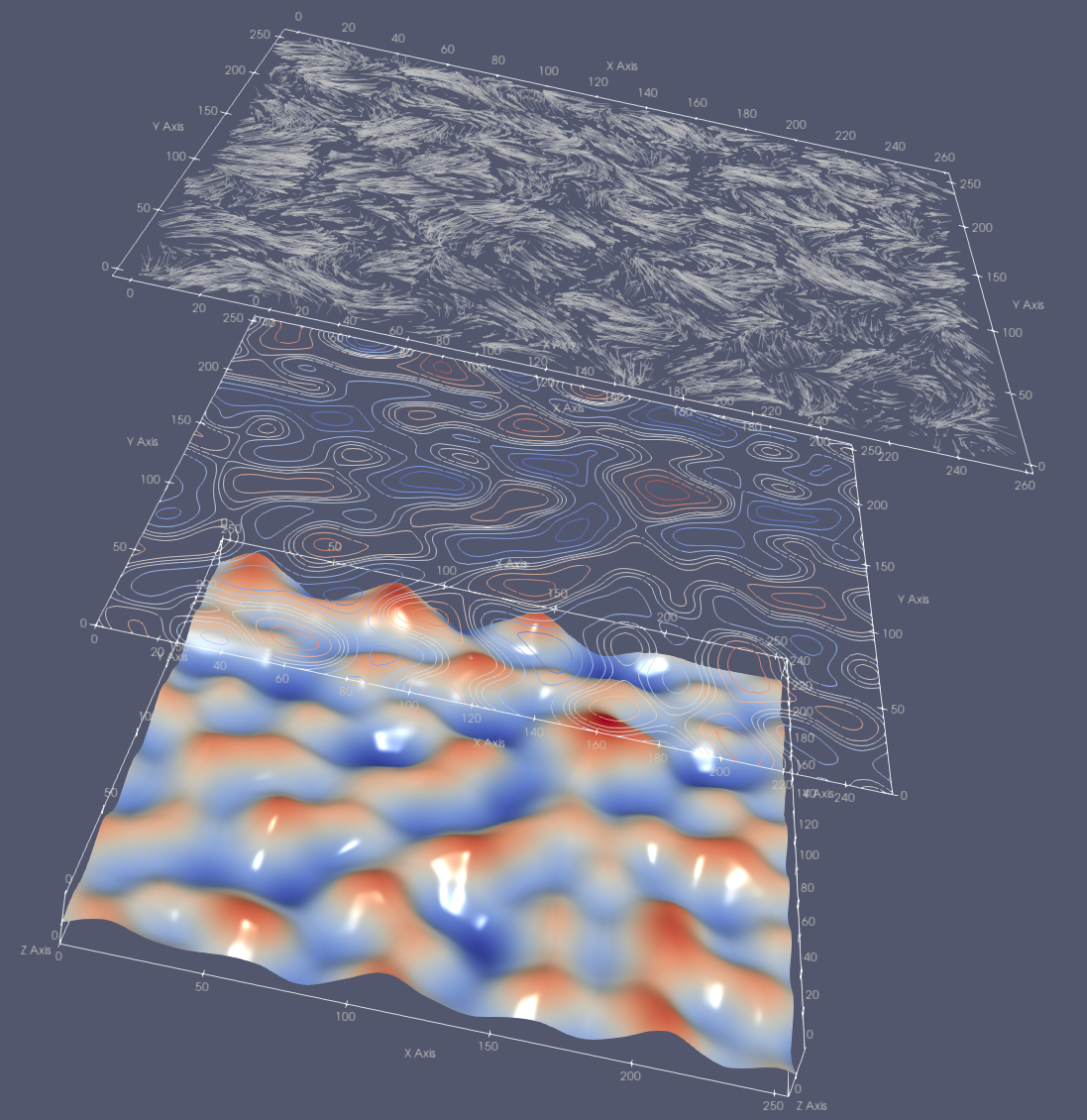
P.47
In this exercise we will generate one scalar and one vector field using perlin noise. The fields can be created by using the following code:
# -*- coding: utf-8 -*-

import numpy as np
import matplotlib.pyplot as plt
import perlin2d as pn
import pyvtk as vtk

if __name__ == "__main__":
    noise = pn.generate_perlin_noise_2d((256, 256), (8, 8)).reshape(256*256,)
    noise_x = pn.generate_perlin_noise_2d((256, 256), (8, 8)).reshape(256*256,1)
    noise_y = pn.generate_perlin_noise_2d((256, 256), (8, 8)).reshape(256*256,1)
The perlin2d module is provided in the assignment. The vector field can be created by combining the noise_x and noise_y using:
vectors = np.hstack((noise_x, noise_y, np.zeros((256*256,1))))
Using the pyvtk module to export the numpy arrays as a 256 x 256 structured points field (vtk.StructuredPoints) with scalars and vector fields attached to the nodes.
Some useful filters are:
WarpByScalar – Warps a 2D field in Z-direction by applying a scale factor. Glyph – Creates a vector field visualization using glyphs. ExtractSurface – Creates a 3D surface from a 2D field. GenerateSurfaceNormals – Calculates Surface normal from a 3D surface. Transform – Translates a node in X, Y, Z direction. Contour - Creates contourlines/surfaces from.
A final visualisation is shown below:
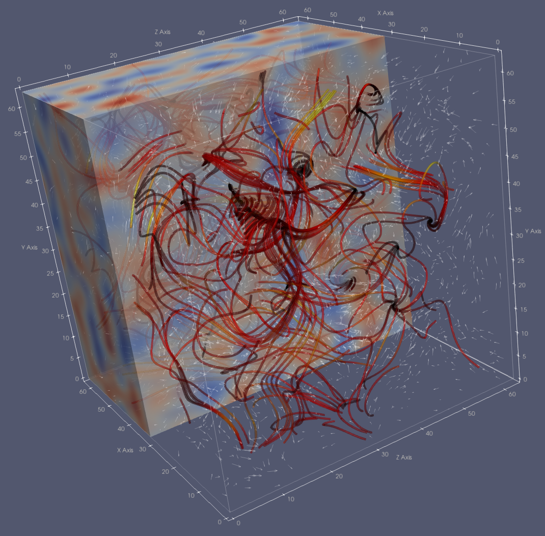
P.48
In this exercise we will generate one scalar and one vector field in 3D using perlin noise. The fields can be created by using the following code:
# -*- coding: utf-8 -*-

import numpy as np
import matplotlib.pyplot as plt
import perlin3d as pn
import pyvtk as vtk

if __name__ == "__main__":
    noise = pn.generate_perlin_noise_3d((64, 64, 64), (8, 8, 8)).reshape(64*64*64,)
    noise_x = pn.generate_perlin_noise_3d((64, 64, 64), (4, 4, 4)).reshape(64*64*64,1)
    noise_y = pn.generate_perlin_noise_3d((64, 64, 64), (4, 4, 4)).reshape(64*64*64,1)
    noise_z = pn.generate_perlin_noise_3d((64, 64, 64), (4, 4, 4)).reshape(64*64*64,1)
The perlin3d module is provided in the assignment. The vector field can be created by combining the noise_x, noise_z and noise_y using:
vectors = np.hstack((noise_x, noise_y, noise_z))
Using the pyvtk module to export the numpy arrays as a 64 x 64 x 64 structured points field (vtk.StructuredPoints) with scalars and vector fields attached to the nodes. An example visualization is shown in the last section.
Some useful filters are:
Glyph – Creates a vector field visualization using glyphs. StreamTracer – Creates stream lines. Use “Seed Type” “Point Source”. Give a radius that covers your data volyme Tube – Attached to a StreamTracer will create solid stream lines, which often look better. Clip - Clips the data volume using a plane. Can be used to see inside.
The final result can look like the following image:
Graph plotter
P.49
In this exercise we will be implementing a graph plotter. We are going to use the Python eval() function to evaluate and plot a Python function. Matplotlib will be integrated in the user interface to implement the plotting of the expression.
Step 1 - Create a form ui-file using Qt Designer / Qt Creator. The following video will show the steps required to create a suitable ui-file. Make sure the controls are given the same names as in the following video:
Step 2 - Download and follow the instructions (Todo) in the template file provided to complete the exercise